Materials
Background and Theory
In just the past few years, astronomers have announced discoveries of at least
250 planets orbiting nearby stars! You can examine the data up close and personal at http://exoplanet.eu These discoveries seem to finally answer the question of whether or not our solar system is unique. We should note, however, that when astronomers state that they have discovered a new planet, what they are really saying is that their data can best be interpreted as a planet orbiting a star. One cannot "prove" that these other planets exist (short of actually going there to explore!); one can only state that, until the hypothesis is disproved, a planet orbiting the star best explains the observations. We cannot see these planets. We can only measure indirectly the influence each one has on its parent star as the star and planet orbit their common center of mass. The planet makes the star "wobble."
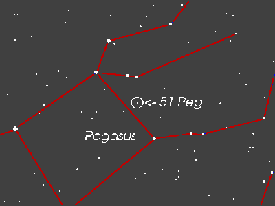
We enter this realm of discovery by working with actual data from observations of the star 51 Pegasi (51 Peg) made at the Lick Observatory in California. These data are the measurements of the Doppler shift of the wavelengths of the absorption lines seen in the spectra of 51 Peg. Table 1 lists the measured radial velocities (RV) as a function of time (recorded in days). As you can see, the radial velocities are sometimes positive and sometimes negative indicating that sometimes the star is receding from (the light is redshifted) and sometimes approaching (the light is blueshifted) our frame of reference. This wobble of the star was the first indication that the star 51 Peg had an invisible companion.
| Day | v (m/s) | Day | v (m/s) | Day | v (m/s) | Day | v (m/s) |
|---|---|---|---|---|---|---|---|
| 0.6 | -20.2 | 4.7 | -27.5 | 7.8 | -31.7 | 10.7 | 56.9 |
| 0.7 | -8.1 | 4.8 | -22.7 | 8.6 | -44.1 | 10.8 | 51 |
| 0.8 | 5.6 | 5.6 | 45.3 | 8.7 | -37.1 | 11.7 | -2.5 |
| 1.6 | 56.4 | 5.7 | 47.6 | 8.8 | -35.3 | 11.8 | -4.6 |
| 1.7 | 66.8 | 5.8 | 56.2 | 9.6 | 25.1 | 12.6 | -38.5 |
| 3.6 | -35.1 | 6.6 | 65.3 | 9.7 | 35.7 | 12.7 | -48.7 |
| 3.7 | -42.6 | 6.7 | 62.5 | 9.8 | 41.2 | 13.6 | 2.7 |
| 4.6 | -33.5 | 7.7 | -22.6 | 10.6 | 61.3 | 13.7 | 17.6 |