$\vec e_1 = (1,0)$
$\vec e_2 = (0,1)$
$\vec e_3 = (-1,0)$
$\vec e_4 = (0,-1)$
$\vec e_5 = (1,1)$
$\vec e_6 = (-1,1)$
$\vec e_7 = (-1,-1)$
$\vec e_8 = (1,-1)$
The goal of this page is to derive an elementary algorithm for modeling fluid flow, starting from only the Boltzmann velocity distribution for ideal gas molecules.
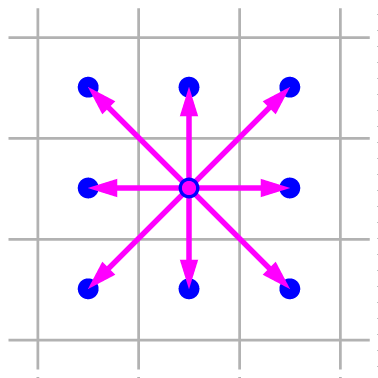
For simplicity I'll work in two dimensions, and discretize space into a square grid or lattice. Each lattice site is big enough to hold a large number of gas molecules, which will be moving in various directions due to their thermal motion plus any large-scale fluid flow. However, I will approximate this rich complexity by allowing only nine different velocity vectors, corresponding to nine elementary displacements during a unit of time: up, down, right, left, along any 45° diagonal, or zero (staying in place). The nine elementary displacements are illustrated and listed below, using a unit system in which the lattice spacing is one unit.
|
$\vec e_0 = 0$ $\vec e_1 = (1,0)$ $\vec e_2 = (0,1)$ $\vec e_3 = (-1,0)$ $\vec e_4 = (0,-1)$ |
$\vec e_5 = (1,1)$ $\vec e_6 = (-1,1)$ $\vec e_7 = (-1,-1)$ $\vec e_8 = (1,-1)$ |
To keep track of how many gas molecules at a site are moving in each of these nine directions, we'll need nine variables. I'll call these variables $n_i$, for $i=0\ldots8$, and define them as the respective densities of molecules with the corresponding velocities. Then the total density $\rho$ of all molecules at any given site is their sum: \begin{equation} \rho = \sum_{i=0}^8 n_i. \end{equation} We can also calculate the macroscopic fluid flow velocity, by taking a weighted average of the nine elementary velocities. I'll call the flow velocity $\vec u$, and use the symbol $c$ for the natural unit of velocity, one grid site per unit time. Then the flow velocity at any given site is \begin{equation} \vec u = \sum_{i=0}^8 \frac{n_i}{\rho} \vec e_i c, \end{equation} which we can write more explicitly as \begin{align} u_x &= \frac{c}{\rho}(n_1 + n_5 + n_8 - n_3 - n_6 - n_7), \\ u_y &= \frac{c}{\rho}(n_2 + n_5 + n_6 - n_4 - n_7 - n_8), \end{align} taking the $x$ and $y$ directions to point rightward and upward, respectively.
The thermal velocities of ideal gas molecules are described by the Boltzmann distribution, which in two dimensions is \begin{equation} D(\vec v) = \frac{m}{2\pi kT} e^{-m|\vec v|^2/2kT}. \label{boltzDist} \end{equation} This is the function that, when integrated over any range of $v_x$ and $v_y$ values, gives the probability of a molecule’s velocity being in that range, where $m$ is the molecule’s mass, $k$ is Boltzmann’s constant, and $T$ is the temperature. The exponent in equation \ref{boltzDist} is the molecule’s kinetic energy, and the prefactor $m/2\pi kT$ ensures that the integral of $D(\vec v)$ over all velocity vectors equals 1 (which you can easily check).